Spurious correlations (or regressions) are widespread, from prestigious academic journals down to newspaper articles. It is important for researchers and data scientists to identify them, and to understand where they are from and how they occur. This post presents 6 major causes of spurious correlations and their implications. They are
Pure coincidence
Trending time series
Sampling bias
Large or massive sample
Data snooping
Selective reporting (fabrication)
Some of them are easy to detect, some are well-known, but some can be quite illusive and even be deceptive.
Pure coincidence
Consider the number of drowning deaths in the U.S. against the number of movies Nicolas Cage appeared from 1999 to 2009.
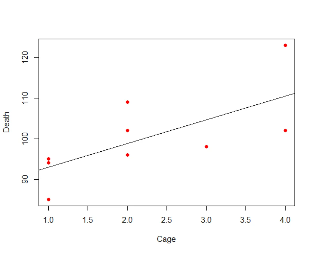
The estimated regression line is Death = 87.13 + 5.82 Cage with the t-statistic of the slope coefficient being 2.68 (p-value = 0.025) and R-square of 0.44. A pure coincidence, but the regression statistics indicate statistical significance, which is simply spurious.
There are many similar examples, often driven by a third factor: e.g., a high correlation between drowning accidents and ice cream sales driven by high temperature.
Trending time series
As widely known in econometrics as spurious regression, a regression with two or more independent random walk time series shows statistically significant slope coefficients, often with high R-square values. The time series Y and X below are two independent random walk series.

The regression results is Y = -0.61 + 0.07 X, with the t-statistic of the slope coefficient being 2.16 (p-value = 0.03).
A special case is where the error term of the regression is stationary, called the cointgration. This special case represents the long-run equilibrium where two or more random walks are driven by a common economic trend. However, if the error term is non-stationary with the properties of a random walk, as in the above example, then it is a spurious regression. A statistically significant correlation occurs simply because they are trending together. Sampling bias The 1936 U.S. Presidential election (Landon vs. Roosevelt) marks the biggest debacle in the history of pre-election polling. The magazine called Literary Digest sent out 10 million questionnaires to the voters sampled from automobile registry and telephone books. Based on 2.5 million responses, the magazine predicted a landslide victory of Landon’s. This prediction was horribly wrong with the outcome being a landslide victory of Roosevelt’s. In contrast, a pre-poll conducted by George Gallup who collected a sample of only 4000 voters made a correct prediction of Roosevelt’s landslide victory.
It turned out that, while Gallup’s poll was based on a random sampling, Literary Digest’s sample was seriously biased. Those who owned telephone or automobile in 1936 was very rich, and those 2.5 million who responded may well have been a small subset of the entire population who were intensely interested in the election.
What is called the found data (“the digital exhaust of web searches, credit card payments and mobiles pinging the nearest phone mast”) widely used in the big data analysis is so messy, noisy, and opaque. It is quite likely that they have serious systematic biases in them, and no one is capable of estimating and controlling such biases, as Harford (2014) points out. The promise of the central limit theorem does not work here, because the way found data was collected is not, by any means, compatible with the assumptions of the theorem. These properties of big data are open to spurious correlations.
Large or massive sample
Consider a regression model: Y = α + β X + u. , the t-statistic for H0: β = 0 can be written as
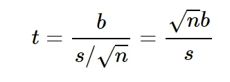
where b is the regression estimate of β, s is an appropriate measure of variability and n is the sample size. It follows from the above expression that, even if the value of b is practically 0, a large enough sample size can make the value of t-statistic greater than 1.96 (in absolute value).
As an example, I consider daily stock return (Y) and sunspot numbers (X) from January 1988 to February 2016 (7345 observations), a relationship with little economic justification. I considered the index returns from 24 stock markets, including Amsterdam, Athens, Bangkok, Brussels, Buenos Aires, Copenhagen, Dublin, Helsinki, Istanbul, Kuala Lumpur, London, Madrid, Manila, New York, Oslo, Paris, Rio de Janeiro, Santiago, Singapore, Stockholm, Sydney, Taipei, Vienna, and Zurich. The total number of pooled observations are 176,280. To highlight the effect of increasing sample size on statistical significance, I conduct pooled regressions by accumulatively pooling the data from the Amsterdam to Zurich markets (increasing the sample size from 7,345 to 176,280).
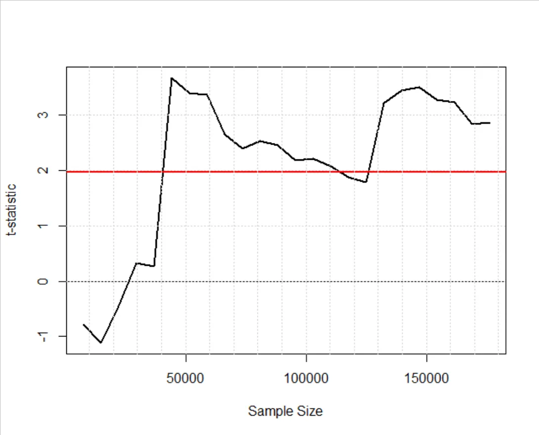
The figure above presents the t-statistic for H0: β = 0 as the sample size increases, with the red line being 1.96. The model becomes statistically significant when the sample size is around 40,000: a statistically significant outcome but a case of spurious correlation. The above regression results are taken from Section 4 of Kim (2017). In fact, the research design follows the study of Hirshleifer and Shumway (2003), who claimed a systematic relationship between stock return and weather in New York.
In this big data era, the use of large or massive sample size is so commonplace, and statistical significance can often be spurious. Data snooping This practice is also known as data dredging, data mining, multiple testing or p-hacking. It generally refers to cherry-picking statistically significant results from a large number of competing empirical models with different sets of predictor variables or samples. This can be done intentionally, but very often unintentionally or even unknowingly to the researchers. If you are testing a correlation at the 5% level of significance, you will have statistically significant results in one in 20 cases as a realization of Type I error, even if there is no relationship. Hence, a spurious correlation can often be the result of this process of cherry-picking, as the cartoon below shows:
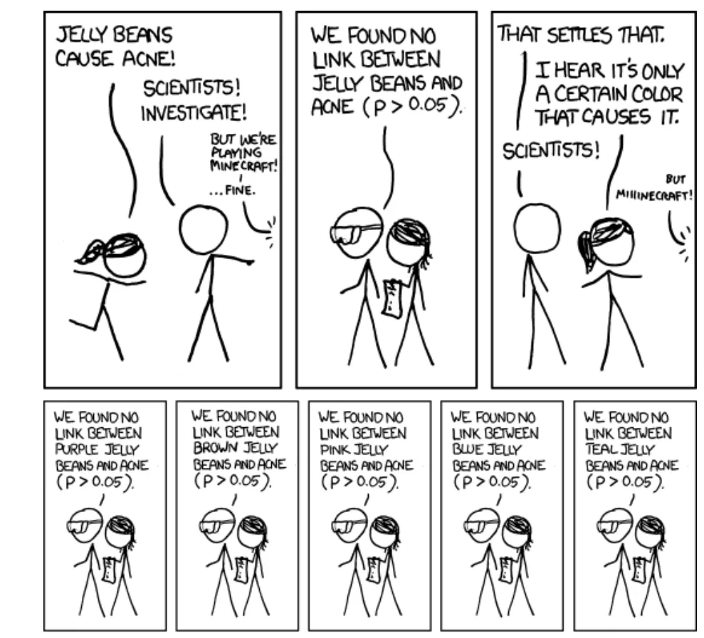
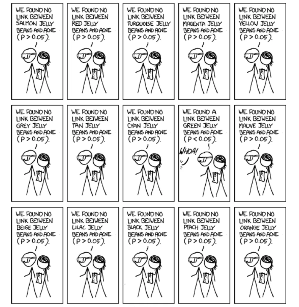
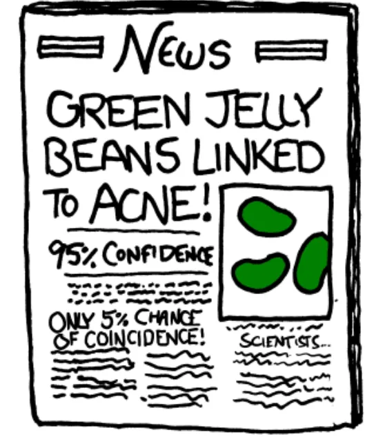
https://iterativepath.wordpress.com/2011/04/07/significance-of-random-flukes/ Selective reporting (fabrication) The spurious correlation can occur as a result of reporting of selective or fabricated results, an unethical practice which cannot be tolerated.
Ancel Keys was one of the most influential scientists of the 20th century. Among his contributions, the most controversial was the Seven Country Study, in which he presented a strong (near perfect) positive relationship between fat intake and heart disease, using a multi-country data set collected in the 1950’s. This result was taken up by the American Heart Assocoiation in the 1970’s, with its official health advice to reduce fat intake in peoples’ diet to avoid heart attacks.
This has changed the world in many ways. The animal fat has been stigmatized as the main cause of heart attacks, and low-fat diet has become a norm for those who seek healthy life and longevity. Food manufacturers around the world have responded to this by supplying low-fat products. In this process, the fat has been removed from food products and replaced with the sugar to maintain the taste and quality.
On the other hand, there are scientists who have claimed that a higher intake of sugar and carbon hydrates, as a result of demonizing the fat, has caused a steep increase of obesity and diabetics since 1990’s. They also refuted the findings of Ancel Keys and argued that sugar has been the main culprit of many deceases. They claim that statistical evidence put forward by Ancel Keys has been fabricated and fudged by selective reporting of the result (to be discussed below).
The controversy still goes on. It seems that the medical world has not fully reached a consensus as to whether the fat is to blame, or sugar, or both, not to mention establishing the compelling medical reasons as to how why fat or sugar is harmful to human body. A big point in this controversy is a suspicion that Ancel Keys presented his findings in a selective way or even fabricated it. He presented Plot A below, while his full data set consists of the data for 22 countries, as in Plot B.
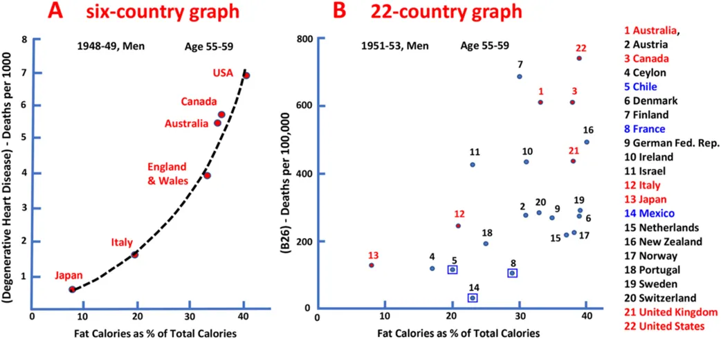
Obesity Reviews, Volume: 22, Issue: S2, First published: 26 January 2021, DOI: (10.1111/obr.13196)
It is not clear if he did it intentionally or he just innocently attempted to highlight his key findings. The bottom line is that his selective reporting has exaggerated the strength of the relationship to the point that the integrity of the whole research is questionable.
A more recent example of research fabrication that shook the world of science can be found here.
I have presented six possible causes of spurious correlation and regression in this post. Accepting the results of spurious correlation represents a Type I error. Incorrect statisitcal decisions can have serious consequences that can affect human lives and welfare of the society. In the big data era where many key decisions are highly data-dependent, we should be aware of these problems and conduct the statistical research in a thoughtful, open, and modest way, as the American Statistical Association recommends.
